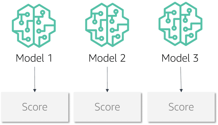
Model:
is a mathematical representation of the learning process. Is a Trained Algorithm used to identify patterns (without rules) in data (trained by ML process) and applied to new data -> prediction
Dataset:
is the data that is collected and used to train, evaluate, and Test the models, collected from many sources, transformed, and pre-processed to use in Machine Learning training. types of data [ Corpus: such as News paper articles]
Data Labeling:
is the target attribute of the data, identifies the value of the dataset related to the machine learning analysis, the label is either provided (supervised), or calculated (unsupervised), a trained model predicts labels on new datasets, Data that is labeled is also called Ground Truth data
Datapoint:
is the coordinate between a feature (x-axis) and a label (y-axis), used to plot a point on the grid (x, f(x))
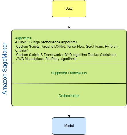
Algorithm:
Defines the structure of an ML model. Is a set of rules or processes used by an AI system to conduct tasks—most often to discover new data insights and patterns, or to predict output values from a given set of input variables. Algorithms enable machine learning (ML) to learn and uses parameters to tune the results.
Framework:
interfaces that allow data scientists and developers to build and deploy machine learning models faster and easier
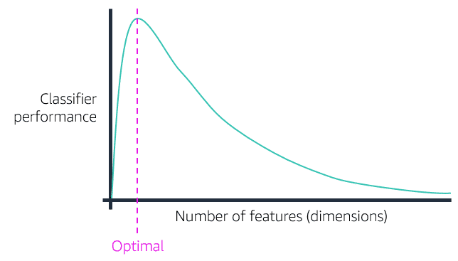
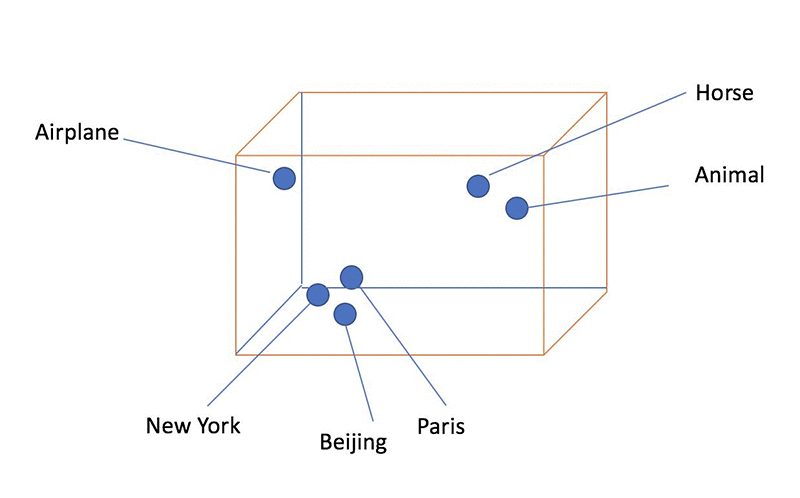
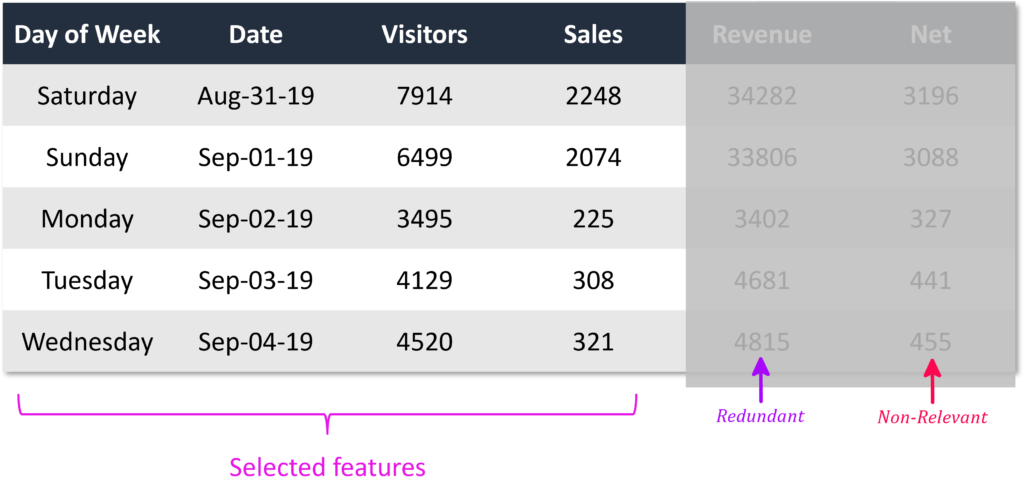
Features (embedding):
parts of the dataset are important to determine the accuracy of the outcome. named feature column, feature variations in (x-axis), example product color, month of the year, stock market value, Features are either [Categorial:=Quality | Continuous:= Quantity] also referred to as embedding, and the number of features in an observation is the dimension
Observations:
The rows, consists of the values of each feature
Prediction (Target value, or label, Estimate):
estimated calculated value as a result of running the model against the real data named Prediction column (y-axis) ex. sales outcome, member enrollments.

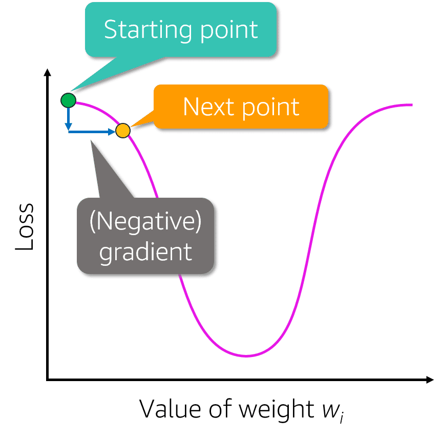
Context
: Weighted features in determining the accuracy.

Where:
x: feature
a: weight – importance

-
-
Supervised:
known inputs/outputs generalize future outputs, Teacher show answer, label data, lead by example, types [Classifications [Binary mapping (T : F) | multi-class mapping (a,b,c …,n)] | Regression no mapping jump value]
-
Unsupervised:
Unknown input/outputs, finds patterns, auto create labels -> clustered data by labeling patterns of data anomaly detection Clustering Algorithm, groups data into different clusters based on similarities in features.
 Anomaly Detection:


-
Reinforcement:
Interacts with the environment, learn to take actions, maximize rewards, continuously improve by feedback from previous (trial/Error) reward/penalty for actions by the agent(driver)
-
Deep Learning:
Based onartificial neurons, Artificial Neural Network (ANN) AI -> rules provided by programmer ML-> Analyzing patterns DL->like human, given basic rules, then iterative complex approach over multiple (100s) of layers and recognize patterns more complex than ML Each layer summarizes and feeds information to the next layer, ultimately producing final output
 Deep Learning Computer Vision
ILSVRC ImageNet Large Scale Visual Recognition Challenge
Deep Learning Computer Vision
ILSVRC ImageNet Large Scale Visual Recognition Challenge
-
# Install Libraries (preinstalled on Sagemaker studio)
%pip install sagemaker boto3 pandas  [ s3fs | "s3fs<=0.4" ] <-- if older pandas
%reset -f <-- restart the kernel
# Install dependencies
import boto3
import pandas as pd
import sagemaker
:
# Load data
df = pd.read_csv("s3://<bucket>/<prefix>/<object>.csv")
# Set up the TrainingInput objects

train_input = TrainingInput(train_path, content_type='text/csv')
validation_input = TrainingInput(validation_path, content_type='text/csv')
# Print data
df
# Configure the estimator
xgb_model = sagemaker.estimator.Estimator(
     image_uri = container,
     role = role,
     instance_count = 1,
     instance_type ='ml.m5.xlarge',
     output_path = output_path,
     sagemaker_session = sagemaker_session,
    rules=[
        Rule.sagemaker(rule_configs.create_xgboost_report())
    ])
# Configure Hyperparameters
xgb_model.set_hyperparameters(
    max_depth = 5,
    eta = 0.2,
    gamma = 4,
    min_child_weight = 6,
    subsample = 0.7,
    verbosity = 0,
    objective = 'binary:logistic',
    num_round = 800)
# Run the training job
xgb_model.fit(
    {
        "train": train_input,
        "validation": validation_input
    },
    wait=True) <-- Takes time
# Evaluate the model
%%capture
time.sleep(500) <--in ms, takes between 3-8 minutes
rule_output_path = xgb_model.output_path + "/" + xgb_model.latest_training_job.job_name + "/rule-output"
! aws s3 ls {rule_output_path} --recursive
! aws s3 cp {rule_output_path} ./ --recursive <-- Takes time wait until report is generated


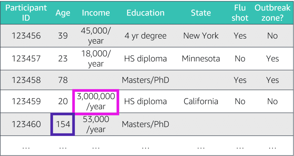
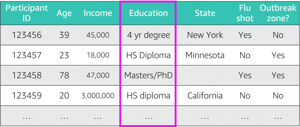
Data Cleaning:
Eliminate inconsistent data (language, format, unit of scale)
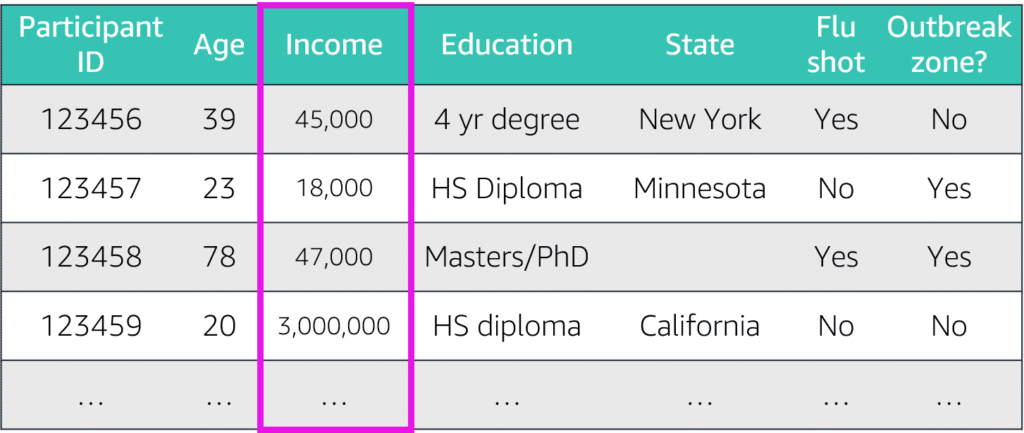
Data Preprocessing
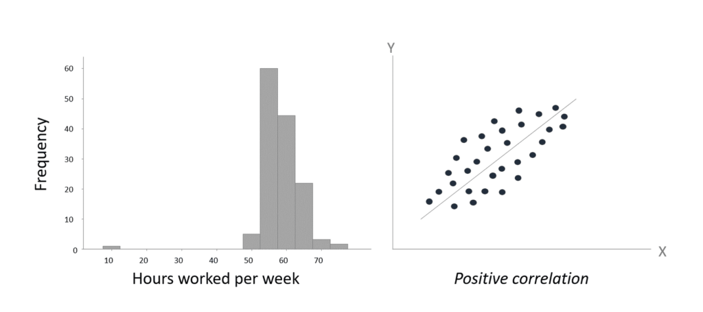
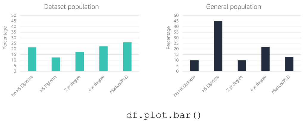
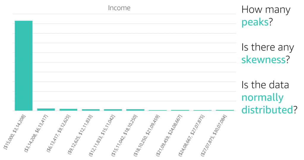
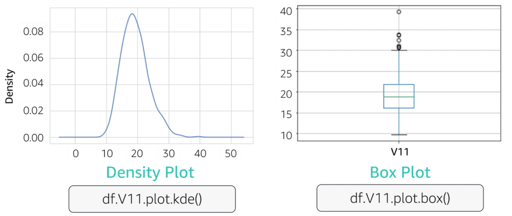
Descriptive Statistics
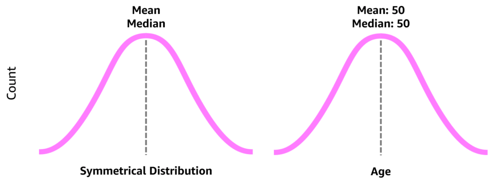
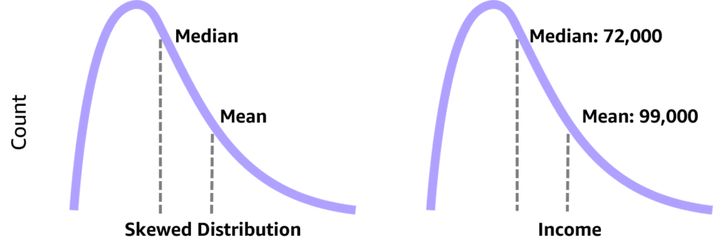
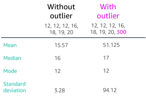
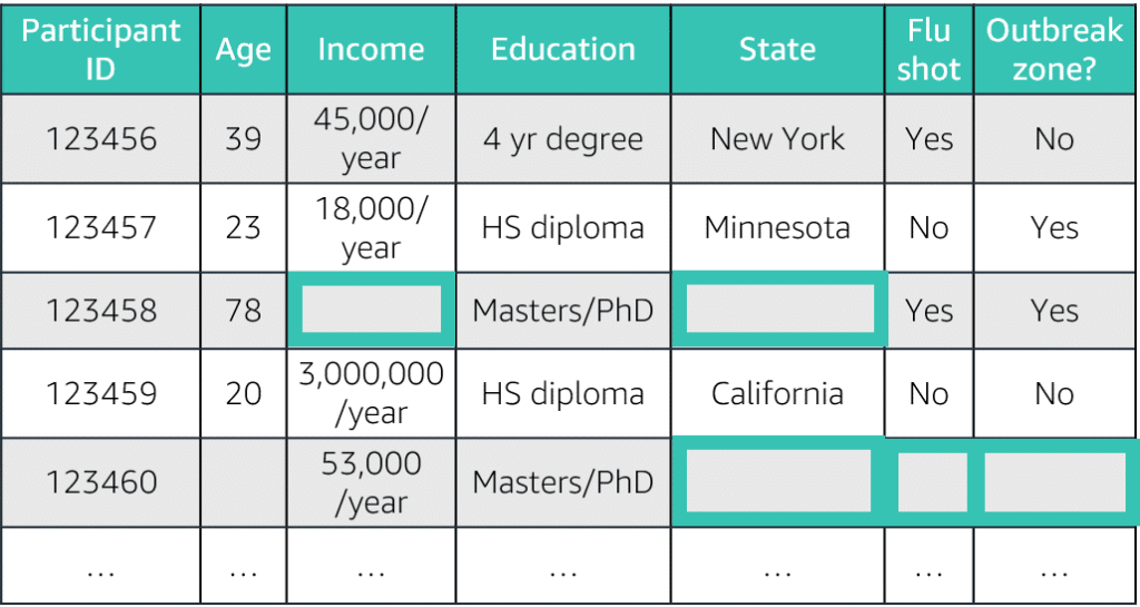
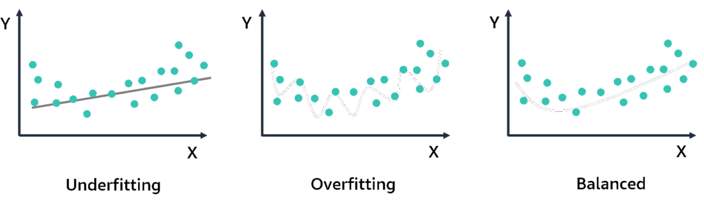
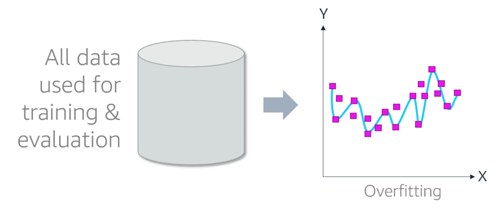
Looks into dataset to discover imbalanced data, use of mean for symmetric data distribution and median for asymmetric data distribution, eliminate outliers data spots (artificial or natural), drop missing data [rows:= not enough samples – overfitting | columns:= underfitting – missing features] or imputing missing values with [ mean | median ]
Medians Is the middle number in a sorted ascending or descending list of numbers and can be more descriptive of that data set than the average, arrange the data points from smallest to largest. If the number of data points is odd, the median is the middle data point in the list. If the number of data points is even, the median is the average of the two middle data points in the list. Used to calculate quarterlies

Where:
q:=quarter i:=1,2,3;
n:= number of samples;
Q:= The order position of the quarterly in the dataset [Q]

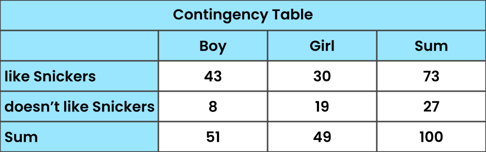


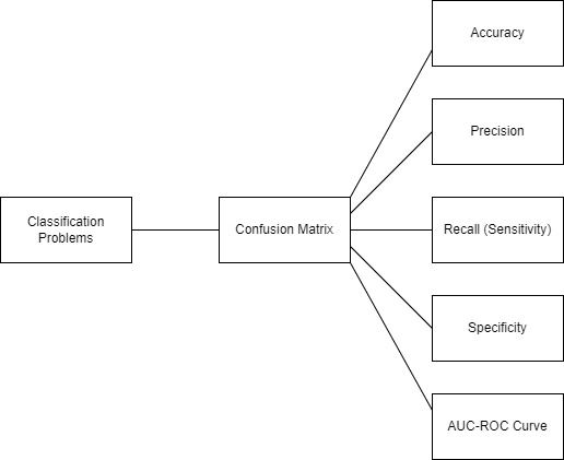


The following metrics can be derived by the confusion metrix:
- Accuracy(score): Less effective lots of TNs, means dataset was easily detect the negatives, unreliable to detect the TPs. The percentage of correct estimates

- Precision: The percentage of correct predicted positives with respect false positives, Best when the cost of FP is high; email scams, investment forecasts, or credit card approvals, ignores the Negatives,

- Recall(Sensitivity): The percentage of correct predicted positives with respect to false negatives. taking into account the false negatives, Used when the cost of FN is high, such as results of medical cancer or tumor exams

- (Specificity): The percentage of correct predicted negatives with respect to false positives. Used when the cost of FP is high, similar to precision but take into account the TN, such as results of elimination voters, or product discontinuation

- F1.Score: Model predictions accuracy, Quantify Precision and Recall in one number, Used for class imbalance (equal number of samples for each class) but want to preserve the equality between precision and recall, binary/multi-class classifications, 1 means all predictions are accurate

Accuracy: All estimates are matched (equally) |
Precision: All Postive Estimates are correct, None is False |
Recall: All Postive Estimates are correct, No False negative estimates |
Specificity: All Negative estimates are correct |
F1 Score: All positive estimates are matched (with impact of All false FP & FN) |

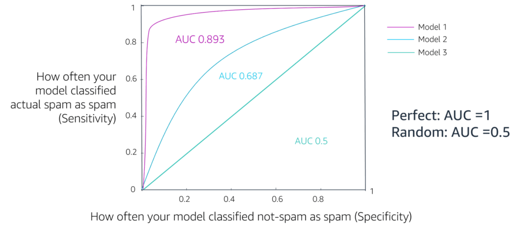
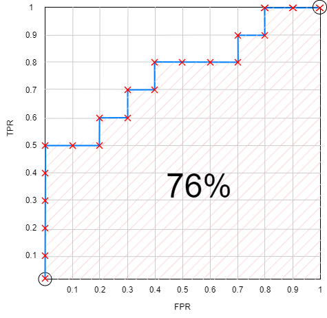
AUC is as the probability that the model ranks a random positive example more highly than a random negative example.
ROC: Receiver Operator Curve,(Recall) the probability curve,
AUC-ROC curve: show what the curve for true positive vs false positive looks like at various thresholds, a threshold is the cut-off probability which determines if the above this threshold the probability is determined to be true otherwise false. the threshold is determined as the point where the curve turns toward FPR (the knee of the curve)
AUC (PR) False Positive Rate (1 – specificity) curve: FP vs TN

*Used when dataset imbalanced skewed to the TN side
ROC True Positive Rate curve (Recall-Sensitivity): TP vs FN 


 The sum of this computed AUC is the AUC in this example 76%.

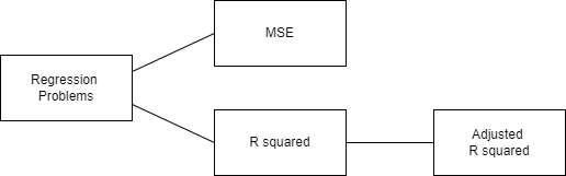
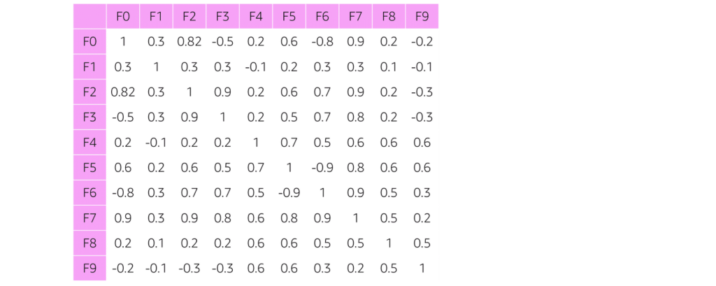
R2 (R squared)
Explains the fraction of variance accounted for by the model, adding more variables increases R, which indicates overfitting, used with regression continuous variables, use Adjusted R2 to address the problem
SSE:=Sum of Squared Error
Adjusted R2
The threshold for a good R squared depends on the the type of business.
Where:
D: Number of data points
V: Number of variables
Random Index
Unsupervised regression metric.


Ordinary Least Squares Regression (OLSR):
A generalized linear modeling technique. It is used for predicting all unknown parameters involved in a linear regression model using one or more dependent parameters, the goal of which is to minimize the sum of the squares of the difference of the observed variables and the explanatory variables.
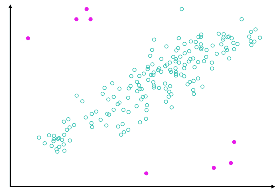
Local Outlier Factor (LOF):
Discover outliers data points before applying dataset to the algorithm
Least-Angel Regression (LARS):
Regression Technique that predicts a dependent variable using one or more independent variables.


Amazon Forecast
Provides forecasts based on historic data, using Deep Learning algorithms, using algorithms such as
- AutoRegressive Integrated Moving Average (ARIMA) based on time series differential, requires small datasets < 100, or
- Prophit fits time series into data by detecting trends at different time intervals works against data irregularities and missing data (seasonal data), Facebook – Neural Prophit adds neural network.
- Amazon DeepAR[+] uses long short-term memory LSTM based on probabilistic sampling techniques splitting the time series into windows(context-length) to predict the forecast horizon. foreword looking.
- Exponential smoothing ETS: statistical algorithm, weighted average of prior features with exponential weight
- The convolutional neural network quantile regression CNN-R: uses causal convolutional networks, doesn’t require future data for the forecast horizon.
- Nonparametric time series (NPTS): used for seasonal data, sparse, or bursty data with a lot of intermitted values
Use Cases:
- Allows addition of weather data
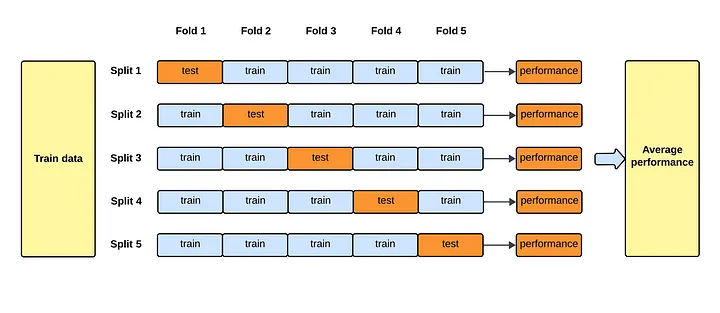
- Data splitting is not possible, use backtesting on historic data (Ground Truth)
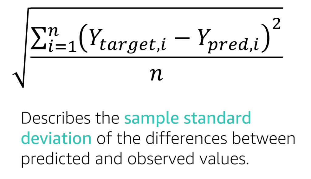
- Measured by RMSE,(to amplify outliers), or Weighted Absolute Percentage Error (WAPE) also known as Mean Absolute Percentage Error (MAPE) or median forecasting

- Quantile based probabilistic, ex. P10:= 10% of real values are less than prediction, for over stocking use higher P.
- Weighted Quantile Loss (wQL) to penalize the model for underfitting versus overfitting to show the over vs under predicting


CatBoost:
open-source implementation of the Gradient Boosting Decision Tree (GBDT) algorithm. GBDT is a supervised learning algorithm that attempts to accurately predict a target variable by combining an ensemble of estimates from a set of simpler and weaker models.
Handles missing values by setting them to 0.
LightGBM:
GBDT is a supervised learning algorithm that attempts to accurately predict a target variable by combining an ensemble of estimates from a set of simpler and weaker models. LightGBM uses additional techniques to significantly improve the efficiency and scalability of conventional GBDT.
Linear Learner:
Linear models are supervised learning algorithms used for solving either classification or regression problems. For input, you give the model labeled examples (x, y). x is a high-dimensional vector and y is a numeric label. For binary classification problems, the label must be either 0 or 1. For multiclass classification problems, the labels must be from 0 to num_classes – 1. For regression problems, y is a real number. The algorithm learns a linear function, or, for classification problems, a linear threshold function, and maps a vector x to an approximation of the label y.
Linear regression:
predicting variable value based on another single variable, numeric value regression
Multivariate regression:
Similar to Linear regression but uses multiple variables to predict a variable value based on multiple variables, numeric value regression
Logistic Regression:
Predicting the probability of an outcome, event, or observation, Binary classification regression
KNN:
The k-nearest neighbors (KNN) algorithm is a non-parametric, supervised learning classifier, which uses proximity to make classifications or predictions about the grouping of an individual data point. Two methods of dimension reduction methods: random projection and the fast Johnson-Lindenstrauss transform. used to find items similarities for recommendation models.
XGBoost – eXtreme Gradient Boosting:
Implementation of the gradient boosted trees algorithm. Gradient boosting is a supervised learning algorithm that tries to accurately predict a target variable by combining multiple estimates from a set of simpler models. accept inferences in text/csv, text/libsvm, recordio-protobuf
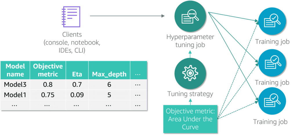
Common XGBoost Hyperparameters:
numclass: The number of classes.
num_round: The number of rounds to run the training.
alpha: L1 regularization term on weights. Increasing this value makes models more conservative..
gamma: Minimum loss reduction required to make a further partition on a leaf node of the tree. The larger, the more conservative the algorithm is.
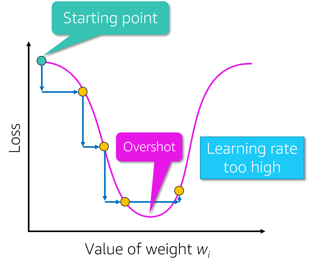
eta: Step size shrinkage used in updates to prevent overfitting. After each boosting step, you can directly get the weights of new features. The eta parameter actually shrinks the feature weights to make the boosting process more conservative.
base_score: The initial prediction score of all instances, global bias..
subsample: Subsample ratio of the training instance. Setting it to 0.5 means that XGBoost randomly collects half of the data instances to grow trees. This prevents overfitting.
Naïve Bayes:
Use principles of probability to perform classification tasks for text categorization problems. use maximum likelihood method
Decision Tree:
Follows a tree-like model of decisions and their possible consequences
Random Forest:
Combines the output of multiple decision trees to reach a single result
Factorization Machines:
The Factorization Machines algorithm is a general-purpose supervised learning algorithm that you can use for both classification and regression tasks. Used to capture interactions between features within high dimensional sparse datasets. For example, in a click prediction system, the Factorization Machines model can capture click rate patterns observed when ads from a certain ad-category are placed on pages from a certain page-category. Factorization machines are a good choice for tasks dealing with high dimensional sparse datasets, such as click prediction and item recommendation.
TabTransformer:
A novel deep tabular data modeling architecture for supervised learning. The TabTransformer architecture is built on self-attention-based Transformers. The Transformer layers transform the embeddings of categorical features into robust contextual embeddings to achieve higher prediction accuracy. The contextual embeddings learned from TabTransformer are highly robust against both missing and noisy data features, and provide better interpretability.![]()

Principal Component Analysis (PCA):
Dimension reduction algorithm, The data is linearly transformed onto a new coordinate system such that the directions (principal components) capturing the largest variation in the data can be easily identified.
K-means clustering:
Partitioning a dataset into a pre-defined number of clusters. useful for tabular data, attempts to find discrete groupings within data, where members of a group are as similar as possible to one another and as different as possible from members of other groups
Linear Discriminant Analysis (LDA):
Finds a linear combination of features that characterizes or separates two or more classes of objects or events. Also known as normal discriminant analysis (NDA), or discriminant function analysis is a generalization of Fisher’s linear discriminant
Latent Dirichlet Allocation (LDA):
Similar to the clustering algorithm K-means, groups words and documents into a predefined number of clusters (i.e. topics). These topics can then be used to organize and search through documents.

BlazingText:
provides highly optimized implementations of the Word2vec and text classification algorithms. The Word2vec algorithm is useful for many downstream natural language processing (NLP) tasks, such as sentiment analysis, named entity recognition, machine translation, etc. Text classification is an important task for applications that perform web searches, information retrieval, ranking, and document classification.
Sequence to Sequence:
Seq2seq is a family of machine learning approaches used for natural language processing. Applications include language translation, image captioning, conversational models, and text summarization. Seq2seq uses sequence transformation: it turns one sequence into another sequence.
Neural Topic Model (NTM):
Organize a corpus of documents into topics that contain word groupings based on their statistical distribution.
Object2Vec:
A Neural embedding algorithm generalizes Word2Vec. It can learn low-dimensional dense embeddings of high-dimensional objects, preserves the semantics of the relationship between pairs of objects, learn by compute nearest neighbors of objects
Text Classification – TensorFlow:
Supports transfer learning with many pretrained models from the TensorFlow Hub. Use transfer learning to fine-tune one of the available pretrained models on your own dataset, even if a large amount of text data is not available. The text classification algorithm takes a text string as input and outputs a probability for each of the class labels. Training datasets must be in CSV format.

Residual Neural Network (ResNet):
The weight layers learn residual functions with reference to the layer inputs. used for Transfer Learning.
Single Shot MultiBox Detector (SSD with VGG):
A single-stage object detection method that discretizes the output space of bounding boxes into a set of default boxes over different aspect ratios and scales per feature map location.

Fully Convolutional Networks (FCN):
They employ solely locally connected layers, such as convolution, pooling and upsampling. Avoiding the use of dense layers means less parameters (making the networks faster to train). It also means an FCN can work for variable image sizes given all connections are local.
Fully Convolutional Networks:
Predict PS propensities based on the integration of residue-level and structure-level features.
DeepAR:
Forecasting scalar (one-dimensional) time series using recurrent neural networks (RNN). Autoregressive integrated moving average (ARIMA) or exponential smoothing (ETS), fit a single model to each individual time series. They then use that model to extrapolate the time series into the future.
Semantic Segmentation:
A deep learning algorithm that associates a label or category with every pixel in an image.


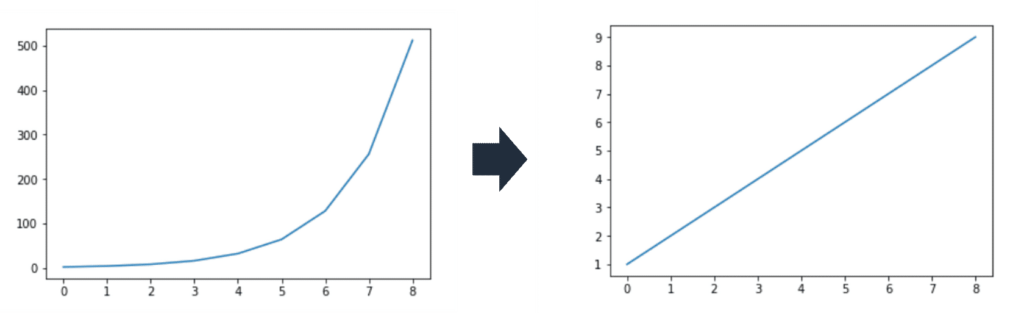
- square/cube root: reduces variance , square works on positive values and zero only, quad works on any value.


- square/cube root: reduces variance , square works on positive values and zero only, quad works on any value.
- Scaling: Convert values into scale 0 . . 1
:Mean/Variance Optimization (MVO):
reduce the impact of outliers

Blends multiple attributes based on Correlation, Smaller values, reduces impact of outliers, values are mean of 0 and standard deviation of 1MinMax:
Best with small standard deviations

Scale values to 0..1, Robust to small standard deviationMaxAbs:
Divide all data into features by the maximum Absolute Value of that feature

Robust:
Substract the median of the features and divides that by the difference between 75th and 25th Quartile
Minimizes impact of large marginal outliers
- Normalizer: Rescales feature values into a range of [0 .. 1], around mean; mean of zero and variance of 1.
- Scaling: Convert values into scale 0 . . 1
Categorial Data Transformation:
Ordinal
Categories ordered and related such as sizes [ S | M | L ] , distances [ near | far], mapped 1 to 1 ex. S = 1, M=5, L=10
Nominal
Categories not ordered and not related such as colors [ Red | Blue | Green ] , Country [ CA | US | MX . . . ]
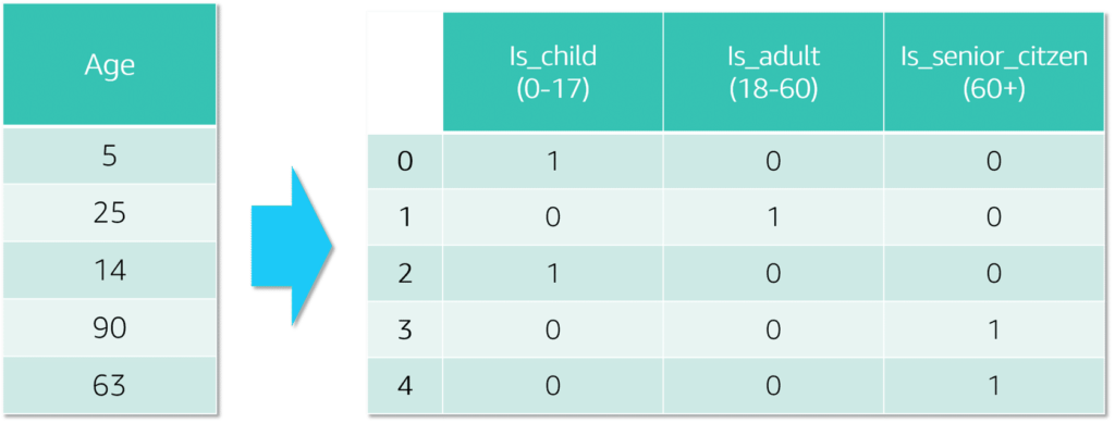
One-hot encoding – each type given its own column values [ 0 | 1 ] for matched values, to reduce number of columns group values by similarities for ex. Territory for countriesCartesian
Takes categorial variables or text as input, and produces new features that capture the interaction between input variables.
N-Gram
Takes a text variable as input and produces strings corresponding to sliding a window of (user-configurable)n words, generating output in the process. An n-gram is a sequence of n words: a 2-gram (which we’ll call bigram) is a two-word sequence of words like “please turn”, “turn your”, or ”your homework”, and a 3-gram (a trigram) is a three-word sequence of words like “please turn your”, or “turn your homework”.
Orthogonal Sparse Bigram (OSB)
Slide the window of size n over the text and outputting every pair of words that includes the first word in the window ex. “The quick brown fox” => {(the,quick) (the,brown) (the,fox)}
Bag of words
NLP algorithm, creates token of the input document text and outputs a statistical depiction of the text such as histograms
Term Frequency-Inverse Document Frequency(tf-idf)
Determines how important a word in a document by giving weights to words that are common and less common in the document (just the count), orderd by weights